This is the first edition in a series of three blog posts that explores the commercial shortcomings of legacy forecast solutions compared to the advantages of Sunairio ONE.
While every business relies on forecasts to some extent, power sector businesses are forecast super-consumers, especially of weather and weather-based forecasts for power demand, wind generation, and solar generation. In fact the growth of renewables has strengthened the link between weather and energy, introducing weather variability to the supply side of the power grid supply-demand balance. This exponentially increases both the requisite forecast complexity of everyday grid operations and the manifest importance of reliable forecasts themselves.
Regardless of their specific role, power-sector forecast consumers fundamentally make quantitative business decisions that rely on weather forecasts. Yet this business need runs straight into two of the most confounding aspects of weather and weather forecasts: the inherent volatility of weather itself and the large uncertainty of weather forecasts.
Most sophisticated weather forecast users have long recognized that the best-practice solution to this problem is to not rely on one forecast, but many. An ensemble approach to forecasting involves issuing many alternative forecasts for the same phenomenon. A common use case is the ubiquitous hurricane track forecast plot that creates an ensemble of many possible trajectories to convey a sense of probabilistic forecast tracks. There are many ways to generate a forecast ensemble and the concept isn’t limited to weather forecasting, but it is widely accepted to be one of the best methods for investigating forecast uncertainty.
Creating an ensemble weather forecast theoretically satisfies two important needs for decision-makers: 1) it theoretically describes the range of possible outcomes, and 2) it can be used to calculate the implied probabilities of all outcomes within the range.
Properly seeing the full range of outcomes – including extreme events – is absolutely critical in power grid applications because extreme events have an outsized effect on reliability and economic outcomes. For example, in the ERCOT real-time power market, just 1% of hours per year account for one-third of total annual market value1. This means that having a clear view of tail risks is paramount for any power grid planner or power market participant, lest they make decisions with a limited forecast set that hides massive risk.
Moreover, it’s important to note that in the context of the modern power grid, extreme events aren’t limited to things like severe storms. Unusual combinations of weather that increase demand while reducing renewable energy generation (such as summer heat that lingers through twilight) is every bit as consequential from a reliability or market perspective.
In this blog post, we evaluate how successful traditional ensemble forecasts and the new Sunairio ONE ensemble are at generating reliable and actionable predictions for power grid/power market applications. We evaluate these ensemble forecasts in three dimensions: calibration (having correct probabilities), sharpness (seeing events clearly), and a new ensemble forecast performance dimension we introduce here: the principle of conspicuous extremes (seeing extreme or tail events).
Ensemble weather forecasts come in many flavors, from the simple historical analogue (a set of historical observations, like historical weather years) to compute-intensive traditional numerical weather prediction (NWP) algorithms, to highly complex deep learning-based generative AI models.
Historical Weather Analogue Ensembles
An historical analogue ensemble of, say, 30 years, constructs a thirty member ensemble where each member of the ensemble is a year of observed weather in the last 30 years. As Historical weather analogues rely on weather observations, serially-complete hourly analogues are generally limited to 75 years or less.
Numerical Weather Prediction Ensembles
Starting from real atmospheric observations, NWPs simulate physical dynamics of the atmosphere to generate a model of future weather. Due to the complex and chaotic nature of atmospheric fluid dynamics, small perturbations in initial weather conditions can lead to dramatically different weather paths. NWP ensembles can take advantage of this by perturbing the initial conditions to simulate an ensemble of “representative” weather realizations. The IFS Ensemble (IFS ENS), an NWP forecast produced by the European Centre for Medium-Range Weather Forecasts (ECMWF), is the gold standard against which all modern weather forecasting systems are compared due to its relatively sharp, skillful short-term forecasts. The IFS ENS consists of one control forecast and 50 additional ensemble paths.
Generative AI Weather Forecast Ensembles
Advances in deep learning have spurred a new paradigm of weather forecasting that borrows ideas from generative AI to produce global weather forecasts that are (1) competitive against the IFS Ensemble and (2) far more computationally efficient. Even without knowing any physical laws, these models, trained on historical reanalysis weather data, produce physically realistic weather patterns. The ECMWF has released an operational ensemble AI weather forecast, the AIFS Ensemble.
The taxonomy of ensemble forecast methods is broad, but many suffer from the same problems: poor calibration, lack of sharpness and poor visibility of extreme events. All of these dimensions are critical for a power sector forecast consumer. A sharp but uncalibrated ensemble will be overly confident but often wrong. A skillful calibrated ensemble that doesn’t satisfy the principle of conspicuous extremes will leave a forecast user exposed to lurking tail risks; you can’t plan for what you can’t see.
Figure 1 illustrates these dynamics. Starting from the left, panel A shows a hypothetical ensemble forecast that is calibrated but not sharp (its implied probabilities are correct but its poor skill means that the ensemble range is very wide), panel B shows an example of an ensemble that is sharp but uncalibrated, while panel C presents an ensemble that is both sharp and calibrated but completely missed an event outright because it does not model extremes. The ensembles in the first two panes have very obvious deficiencies while the ensemble in the third pane exposes the forecast user to more insidious risks – the forecast looks reasonable, performs well in normal weather conditions, but quietly hides tail risks.
Panel D, on the other hand, depicts an ideal ensemble forecast: sharp, calibrated, and extremes-conspicuous.

Figure 1. In the first three panes we show three hypothetical 50 path forecast ensembles that each suffer in one of the three forecast performance dimensions: calibration, sharpness and the principle of conspicuous extremes. In the third, we show an ideal ensemble with 10x as many paths. It is just as sharp as panel C but with more paths, capturing the tails of the distribution.
As we show in this blog post, legacy ensemble forecasts commonly exhibit the deficiencies shown above in A-C, while the new Sunairio ONE method is intelligently designed to replicate the ideal ensemble paradigm in D.
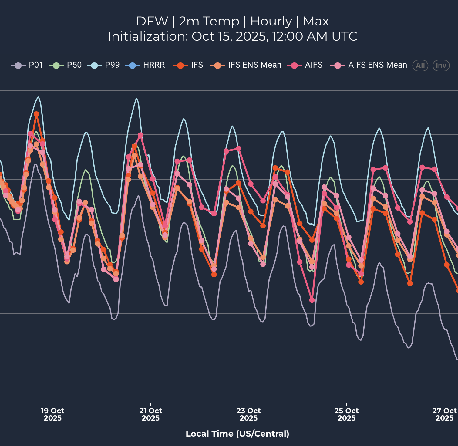
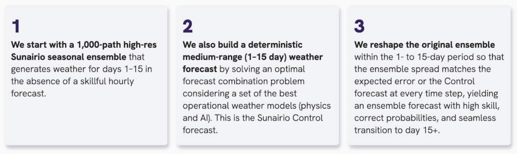
Created in response to the significant limitations of the traditional ensemble forecast classes, Sunairio ONE is powered by a hybrid forecast architecture and designed to maximize commercial actionability. The ONE forecast begins by creating a 1,000-path weather ensemble via a long-range generative weather algorithm that samples from known distributions. Within the medium range window (1-14 days), a deterministic Control forecast is then created by solving an optimal forecast combination problem given the most recent public model guidance. Finally, the original seasonal ensemble is reshaped – conditional on the Control forecast – such that the expected ensemble forecast error matches the ensemble spread.
In the following sections we compare the ensemble forecast of Sunairio ONE to benchmark models in applications for both short and long range forecasting.
Long-range Forecasts
Over longer time horizons (months to years), use of the Historical Analogue approach for ensemble forecasting in the power sector is commonplace as there are no skillful hourly weather forecasts. Accordingly, we compare how well Sunairio ONE performs over a long lead time by examining its performance against a 74-year Historical Analogue. As Figure 2 shows, we plot the ensemble calibration of Sunairio ONE against the Historical Analogue for a 12-month forecast that was issued with 6-18 months forecast lead time, using Daily Maximum Temperatures at Philadelphia airport (PHL). This type of plot, known as a probability-probability (PP) plot, compares the implied ensemble event probability (x-axis) to the actual observed event frequency (y-axis). As the plot shows, a 74-year historical ensemble is poorly calibrated (note how it generally underpredicts the probability of daily maximum temperatures– is biased low–a result of not adjusting for climate change), while the Sunairio ONE ensemble closely hews to the 1:1 line that represents good calibration: implied ensemble forecast probabilities = observed frequencies.
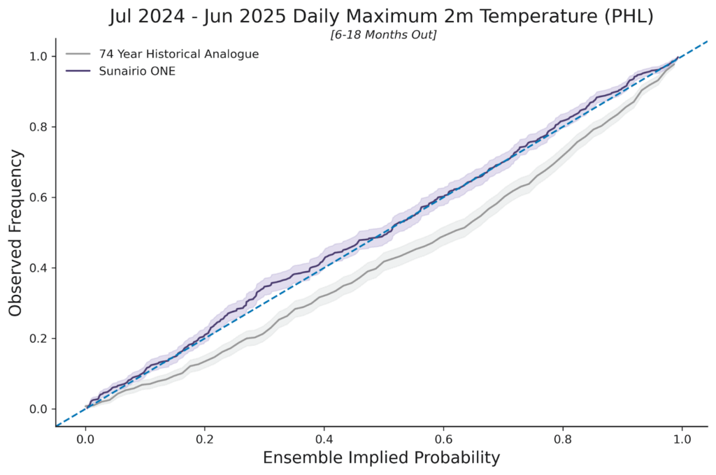
Figure 2. PP plot of 74-year Historical Analogue ensemble and Sunairio ONE for daily maximum temperature for the period July 2024 to June 2025. Historical Analogue for the years 1950-2023. Sunairio ONE trained through 2023 and then predicted for the Jul-24 to Jun-25 period (6 to 18 months forecast lead time)
The Historical Analogue approach also performs poorly when considering its ability to see extremes. As Table 1 shows, the 74-year Historical Analogue completely missed 184 hours per year within the analogue range (a forecast surprise), as there are simply too few samples (74) to accurately represent the range of likely weather over an 8,760 hourly period. By contrast, Sunairio ONE captures 97% of those missed extreme values (178 of the 184 misses) due to the more robust 1,000-member ensemble that’s capable of seeing well past 99th percentile events.
|
# of Hourly 2m Temperature Surprises, PHL July 2024 - June 2025 | |
|---|---|
| 74 Year Historical Analogue (1950-2023) | 184 |
| Sunairo ONE (6-18 months out) | 6 |
Table 1. Hourly 2m temperature surprises at PHL for the period July 2024 to June 2025 from two different approaches to long-range ensemble forecasting
Short- and Medium-range Forecasts
Over shorter time horizons we compare Sunairio ONE to benchmark medium-range (14-day) public ensemble forecast models. As Figure 3 shows, Sunairio ONE again outperforms traditional benchmarks such as the ECMWF’s IFS Ensemble by generating a calibrated forecast – even through the upper quartile event range (events in the 75th to 100th percentile). As we see, Sunairio ONE replicates extreme events at the correct observed frequencies while the IFS Ensemble (the gold standard NWP ensemble) drastically underpredicts them.
For example, the dotted green line indicates that temperatures predicted by the IFS Ensemble to occur no more than 5% of the time (the 0.95 non-exceedance probability level) actually occurred more than 21% of the time (a non-exceedance frequency of about 0.79), meaning that the these temperature events were about 4 times more likely than the IFS ensemble implied.
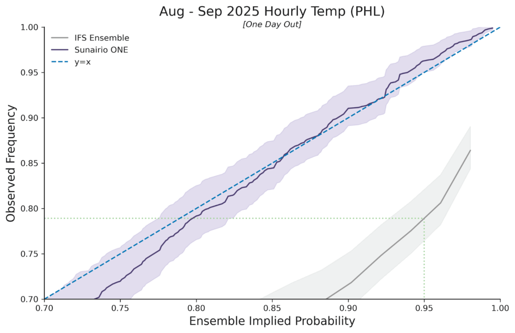
Figure 3. PP plot of Sunairio ONE and the IFS Ensemble for hourly temperature at PHL. PP plot is zoomed in to the upper quartile. Dotted green line shows that the IFS Ensemble p95 level is actually the observed p79 frequency.
Moreover, Sunairio ONE isn’t just calibrated – it’s also demonstrably sharper than traditional ensemble forecasts. Comparing the continuous ranked probability score (CRPS – a metric used to evaluate the accuracy of a probabilistic forecast) of Sunairio ONE to the GFS Ensemble (known as GEFS, NOAA’s benchmark medium-range forecast ensemble) we see that Sunairio ONE improves CRPS across a suite of weather variables by 20% or more (Figure 4).
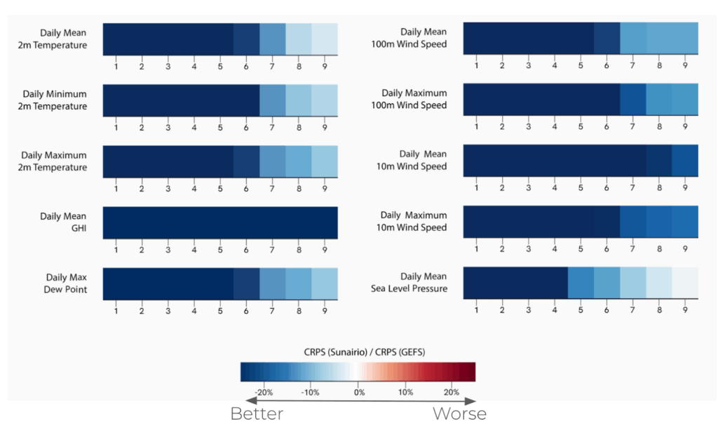
Figure 4. Relative improvement in CRPS for Sunairio ONE compared to GEFS across several weather variables and daily aggregations.
The Sunairio ONE ensemble also does a much better job at seeing extreme events than traditional forecasts. Here we note that traditional weather forecasts actually tend to be worse at seeing extremes the closer they are to happening. For example, Figure 5 plots the number of hourly temperature forecast surprises (events in which the actual temperature realized completely outside of the ensemble range) for the IFS Ensemble at PHL over a period from June 20 to September 22, 2025 – with just one day of lead time. That is, we collected IFS Ensemble temperature forecasts for the following calendar day every day during this period and counted the number of hours in which hourly temperatures realized above or below the 51-member ensemble set.
Over this 95-day period, there were a total of 412 hourly forecast surprises (including misses above and below the ensemble range). Notably, the IFS Ensemble was nearly perfectly unbiased during this period at PHL, with MBE measuring +0.02 deg F, meaning the misses were not caused by the ensemble range being systematically shifted up or down. Rather, the forecast was simply overconfident (and wrong). We do not show the Sunairio ONE forecast surprises in this plot because the Sunairio ONE ensemble did not miss any hours.
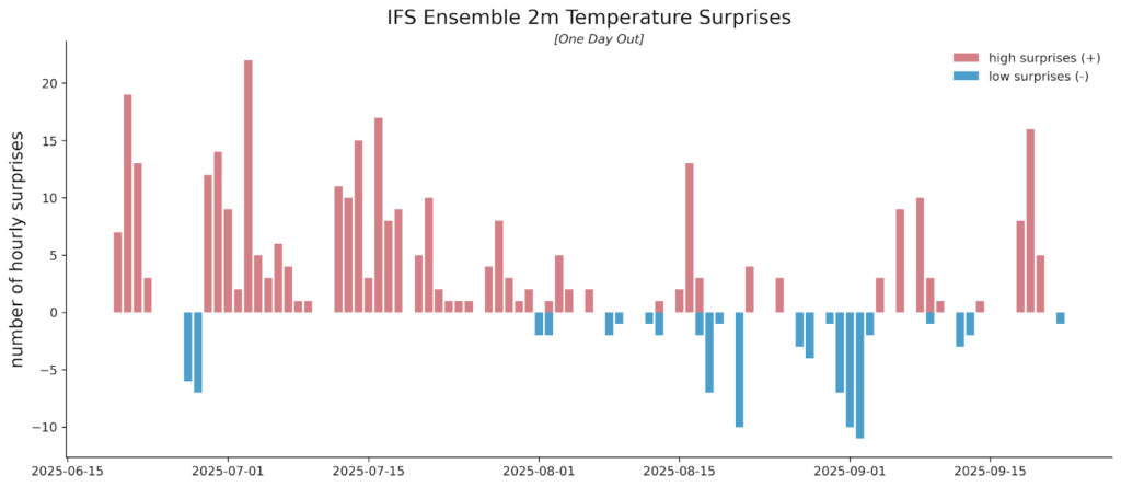
Figure 5. Daily counts of hourly forecast surprises (hourly realizations outside the 51-member ensemble range) for the IFS Ensemble, June 20 to September 22, 2025 at PHL, with one day of forecast lead time.
Next we measure the forecast surprises on daily maximums and daily minimums for 1 day, 7 days, and 14 days forecast lead time and compare them to the number of forecast surprises that should be expected given the ensemble size. Table 2 presents the results. As the table shows, the IFS Ensemble missed 3 daily max/min events at 14 days and 8 daily max/min events at 7 days (compared to an expected range of 2 to 6), but missed a whopping 17 days (18.5% of the analyzed period) at just 1 day of forecast lead time. This data suggests that the IFS Ensemble has an inherent underdispersion weakness which becomes more profound as the forecast lead time decreases.
To estimate the magnitude of the underdispersion, we calculate how much wider the ensemble would have to be so that the actual misses fall within the expected range. As the table shows, the underdispersion is at least 1 deg F at 7 days of lead time and more than 3 degrees at 1 day of lead time.
| Lead | Sunairio ONE exp. # surprises | Sunairio ONE # surprises | IFS ENS exp. # surprises | IFS ENS # Surprises | IFS ENS Underdispersion |
|---|---|---|---|---|---|
| 1 day | 0 to 1 | 0 (0%) | 2 to 6 | 17 (18.5%) | > 3F |
| 7 days | 0 to 1 | 0 (0%) | 2 to 6 | 8 (8.6%) | > 1F |
| 14 days | 0 to 1 | 0 (0%) | 2 to 6 | 3 (3.3%) | 0F |
Table 2. Expected forecast surprises, actual forecast surprises, and estimated underdispersion for Sunairio ONE and the IFS Ensemble. 2m temperature daily maximum and daily minimum forecasts at PHL, one day forecast lead time, June 16 to September 28, 2025.
Forecast surprises such as these have immense consequences for power grid operators and power market participants because they represent hidden risks that generally haven’t been accounted for in any decision-making. That is, traditional ensemble weather forecasts, especially those issued for the next calendar day, are commonly thought to encapsulate a complete range of risk–but they do not.
In fact as the left column of Figure 6 shows, during a three-day period from September 26 to 28 this year the IFS Ensemble range missed each day’s maximum temperature just one day out. There are 51 ensemble members within the IFS ENS and not a single one was high enough.
Comparing that performance to Sunairio ONE (right column of Figure 6), we see that while the realized temperature was indeed towards the upper range of our one-day forecast, it was well within the ensemble spread–visible to any forecast user making quantitative scheduling, dispatching, or trading decisions.
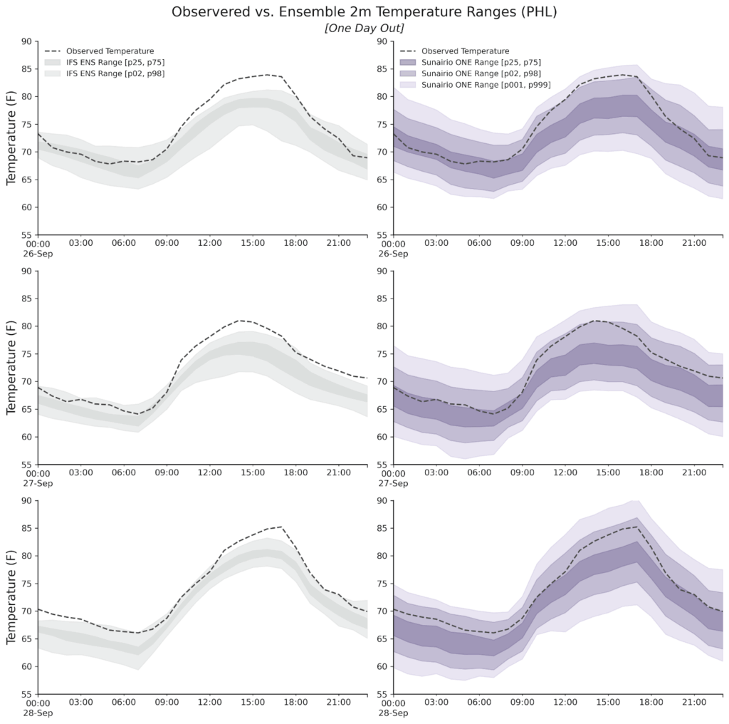
Figure 6. One day lead time 2m temperature forecast ensemble range for IFS Ensemble (left) and Sunairio ONE (right), along with observations. PHL airport, September 26-28, 2025.
As these plots show, Sunairio ONE ensembles exhibit the overall characteristics of the ideal ensemble forecast from Figure 1: calibrated, sharp, and showing the risk of extremes.
To put the IFS Ensemble forecast surprises in context of power grid balances, we convert the temperature misses seen here into hidden PJM load risks (assuming a similar temperature surprise across the PJM footprint). Figure 7 plots the result, showing that a ~2-4 deg F temperature miss across these hours accounts for up to 6 GW of hidden load risk–equivalent to the regional power demand of the entire Philadelphia metro area!
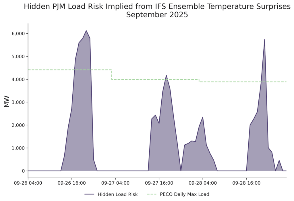
Figure 7. Magnitude of potential hidden PJM load due to IFS Ensemble temperature surprises, September 26-28, 2025, and daily max load for PECO (Philadelphia Electric Company).
This means that a major city’s worth of demand risk was hiding in plain sight, invisible to forecast users because the benchmark models fail to see extremes – even just one day out.
Ensemble forecasts are critical tools for grid operators, power market participants, and other decision-makers in the energy sector. However, legacy ensemble forecast methods suffer from chronic and significant deficiencies that obscure important risks: missing hundreds of hours per year, misrepresenting event probabilities by a factor of 4, and hiding extreme events equivalent to a city’s-worth of power demand.
Sunairio ONE addresses these problems by intelligently generating an ensemble forecast that’s calibrated, sharp, and sees the all-important extreme events.