Sometimes the interactions between renewable energy and energy markets are so complex that it’s helpful to simplify the dynamics with relatable analogies. So for this blog post we’re going to start by telling a story about a wheat farm instead of a wind or solar farm. And in doing so we’ll expose one of the most important but subtle risks to utility-scale renewable energy asset profitability.
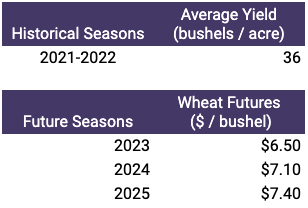
Our story begins with a hypothetical wheat farm investor who is evaluating the purchase of a 100 acre wheat farm. The wheat farm investor is presented with some historical data of average crop yield for similar farmland and the current wheat futures prices. The data shows the following:
The farmland in question is being offered for a price that implies a $20,000 per year operating cost. Using this data, the farmer constructs a financial model of the wheat farm with two assumptions:
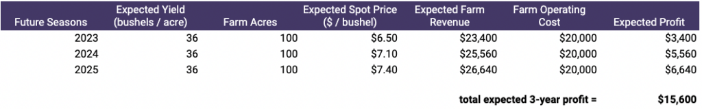
Under these assumptions, this looks like a profitable investment!
The wheat farmer decides to purchase the farm and grow wheat. Traveling in time to the end of 2025, here’s what happens:
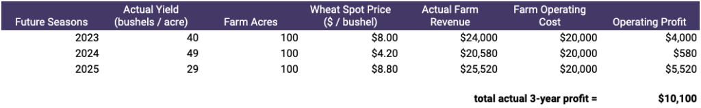
She made less money than she expected, and she almost lost money in 2024 despite having a bumper crop. This happened because everybody else growing wheat had a bumper crop in 2024 as well, which negatively affected market prices due to supply and demand balances. Furthermore, when her crops suffered and she underproduced in 2023 and 2025, everybody else did, too. This caused supply to drop and market prices to rise relative to the expected price from the futures contract.
Perhaps most surprisingly, the quantity and price outcomes were equivalent to expectations when looking at a multi-year average:

The average crop yield over the three year period matches the historical crop yield average, and the average spot price of the three year period matches the average of the futures prices when she bought the farm. Her assumptions of expected yield and price over the three year period were correct.
However, the farm realized lower revenue than expected because of the relationship between seasonal yield and prices: in good growing seasons when there’s a bumper crop, the farmer has more wheat to sell, but at low prices. On the other hand, during poor growing seasons prices are higher because supply is low–but in those seasons the farm brings less crop to market. This negative correlation between yield and price– and the variability between each market phase–eats away at the farm’s profitability.
It turns out that wind farm and solar farm owners experience the same phenomenon in energy markets, except that the comparable “season” in energy markets occurs (at least) every hour when wind or solar energy is generated and energy prices are set by the grid operator.
For example, a merchant wind farm owner might naively think that high wind hours are great for their asset, while low wind hours are worse. This could be the case…unless the wind farm’s generation is highly correlated with the generation from a lot of other wind farms. In that case, when it’s blowing a lot at one farm…it’s probably blowing a lot at other wind farms, leading to excess regional wind generation and low spot prices.
What this means is that using expected generation levels and expected price levels to value the variable energy from wind farms and solar farms leads to overestimates of actual project revenues.
We’ve heard this concept referred to by a number of names including variable generation risk (VGR) and cannibalization. Regardless of what we call it, it can be a major problem for renewable energy investors (who realize lower revenues compared to pre-construction expectations) and it’s not a trivial thing to predict. In fact it’s not uncommon to come across particularly affected projects that can experience VGR costs of as much as 10% or higher of their annual revenue. Moreover, we expect VGR to change dramatically in markets where installed renewables capacity is increasing significantly.
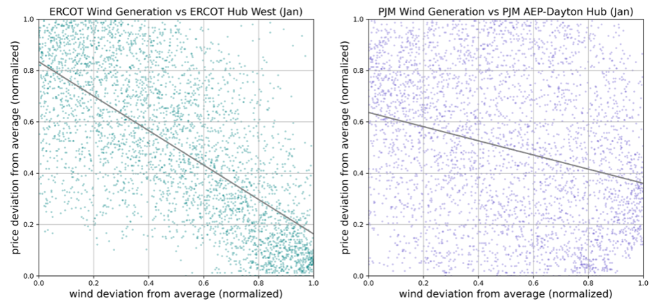
As an example of how this dynamic changes over time as the grid mix changes, here are plots of hourly wind generation levels versus hourly price levels for ERCOT and PJM. For each chart we’ve normalized the wind generation and prices to plot deviations from expected values. You can clearly see this negative relationship is stronger in regions that have a higher share of installed wind capacity than others. (ERCOT > PJM) Over time, these relationships change as the grid mix changes.
Anyone who’s exposed to quantity and price risk through an investment in renewables needs to be familiar with this concept. Importantly, that also extends to buyers of financial PPAs, such as those being sold to corporates to help underwrite new utility-scale projects. Financial PPA buyers wear this risk and therefore it’s essential for them to understand its effect on future contract settlement ranges and terminal contract value.
We’ll explore these issues in more detail, including strategies to mitigate these risks, in future posts.